Kohonen

Introduction

The cerebral cortex is arguably the most fascinating structure in all of human physiology. Although vastly complex on a microscopic level, the cortex reveals a consistently uniform structure on a macroscopic scale, from one brain to another. Centers for such diverse activities as thought, speech, vision, hearing, and motor functions lie in specific areas of the cortex, and these areas are located consistently relative to one another. Moreover, individual areas exhibit a logical ordering of their functionality. An example is the so-called tonotopic map of the auditory regions, where neighboring neurons respond to similar sound frequencies in an orderly sequence from high pitch to low pitch. Another example is the somatotopic map of motor nerves. Regions such as the tonotopic map and the somatotopic map can be referred to as ordered feature maps. The purpose of this chapter is to investigate a mechanism by which these ordered feature maps might develop naturally.
It appears likely that our genetic makeup predestines our neural development to a large extent. Whether the mechanisms that we shall describe here play a major or a minor role in the organization of neural tissue is not an issue for us. It was, however, an interest in discovering how such an organization might be learned that led Kohonen.
The cortex is essentially a large (approximately 1-meter-square, in adult humans) thin (2-to-4-millimeter thick) sheet consisting of six layers of neurons of varying type and density. It is folded into its familiar shape to maximize packing density in the cranium. Since we are not so much concerned with the details of anatomy here, we shall consider an adequate model of the cortex to be a two-dimensional sheet of processing elements.
As a simplified definition, we can say that, in a topology-preserving map, units located physically next to each other will respond to classes of input vectors that are likewise next to each other. Although it is easy to visualize units next to each other in a two-dimensional array, it is not so easy to determine which classes of vectors are next to each other in a high-dimensional space. Large-dimensional input vectors are, in a sense, projected down on the twodimensional map in a way that maintains the natural order of the input vectors. This dimensional reduction could allow us to visualize easily important relationships among the data that otherwise might go unnoticed. In the next section, we shall formalize some of the definitions presented in this section, and shall look at the mathematics of the topology-preserving map. Henceforth, we shall refer to the topology-preserving map as a self-organizing map (SOM).
The Kohonen network (Kohonen, 1982, 1984) can be seen as an extension to the competitive learning network, although this is chronologically incorrect. Also, the Kohonen network has a diferent set of applications.In the Kohonen network, the output units in S are ordered in some fashion, often in a twodimensional grid or array, although this is application-dependent. The ordering, which is chosen by the user1, determines which output neurons are neighbours.
Now, when learning patterns are presented to the network, the weights to the output units are thus adapted such that the order present in the input space ℜN is preserved in the output, i.e., the neurons in S. This means that learning patterns which are near to each other in the input space (where 'near' is determined by the distance measure used in finding the winning unit)
must be mapped on output units which are also near to each other, i.e., the same or neighbouring units. Thus, if inputs are uniformly distributed in ℜN and the order must be preserved, the dimensionality of S must be at least N. The mapping, which represents a discretisation of the input space, is said to be topology preserving. However, if the inputs are restricted to a subspace of ℜN, a Kohonen network can be used of lower dimensionality. For example: data on a twodimensional manifold in a high dimensional input space can be mapped onto a two-dimensional Kohonen network, which can for example be used for visualisation of the data. Usually, the learning patterns are random samples from ℜN. At time t, a sample x(t) is generated and presented to the network. Using the same formulas as in section 6.1, the winning unit k is determined. Next, the weights to this winning unit as well as its neighbours are adapted using the learning rule

Here, g(o,k) is a decreasing function of the grid-distance between units o and k, such that g(k,k) = 1. For example, for g() a Gaussian function can be used, such that (in one dimension!) g(o,k) = exp -(-(o - k)2).Due to this collective learning scheme, input signals.

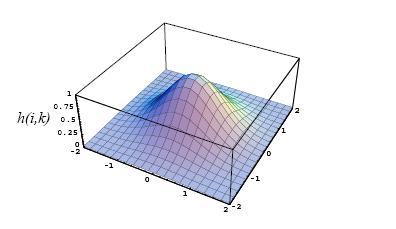
Gaussian neuron distance function g(). In this case, g() is shown for a two-dimensional grid because it looks nice. which are near to each other will be mapped on neighbouring neurons. Thus the topology inherently present in the input signals will be preserved in the mapping, such as depicted in figure

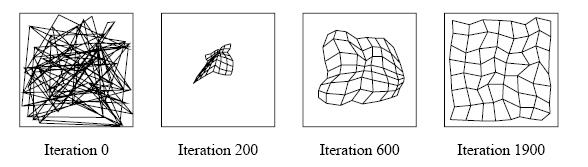
A topology-conserving map converging. The weight vectors of a network with two inputs and 8x8 output neurons arranged in a planar grid are shown. A line in each figure connects weight wi(o1,o2) with weights wi(o1+1,o2) and wi(i1,i2+1). The leftmost gure shows the initial weights; the rightmost when the map is almost completely formed.
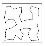
If the intrinsic dimensionality of S is less than N, the neurons in the network are 'folded' in the input space, such as depicted in figure

The topology-conserving quality of this network has many counterparts in biological brains. The brain is organised in many places so that aspects of the sensory environment are represented in the form of two-dimensional maps. For example, in the visual system, there are several topographic mappings of visual space onto the surface of the visual cortex. There are organised mappings of the body surface onto the cortex in both motor and somatosensory areas, and tonotopic mappings of frequency in the auditory cortex. The use of topographic representations, where some important aspect of a sensory modality is related to the physical locations of the cells on a surface, is so common that it obviously serves an important information processing function.
It does not come as a surprise, therefore, that already many applications have been devised of the Kohonen topology-conserving maps. Kohonen himself has successfully used the network for phoneme-recognition (Kohonen, Makisara, & Saramaki, 1984). Also, the network has been used to merge sensory data from di erent kinds of sensors, such as auditory and visual, 'looking' at the same scene (Gielen, Krommenhoek, & Gisbergen, 1991).
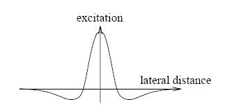
To explain the plausibility of a similar structure in biological networks, Kohonen remarks that the lateral inhibition between the neurons could be obtained via e erent connections between those neurons. In one dimension, those connection strengths form a 'Mexican hat'
Mexican hat. Lateral interaction around the winning neuron as a function of distance: excitation to nearby neurons, inhibition to farther of neurons.

The SOM Learning Algorithm

During the training period, each unit with a positive activity within the neighborhood of the winning unit participates in the learning process.We can describe the learning process by the equations:

wi = α(t)(x - wi,)U(Yi)

where w, is the weight vector of the ith unit and x is the input vector. The function U(yi) is zero unless yi > 0 in which case U(yi) = 1, ensuring that only those units with positive activity participate in the learning process. The factor α(t) is written as a function of time to anticipate our desire to change it as learning progresses. To demonstrate the formation of an ordered feature map, we shall use an example in which units are trained to recognize their relative positions in two-dimensional space.
Each processing element is identified by its coordinates, (u,v), in two-dimensional space. Weight vectors for this example are also two dimensional and are initially assigned to the processing elements randomly. As with other competitive structures, a winning processing element is determined for each input vector based on the similarity between the input vector and the weight vector. For an input vector x, the winning unit can be determined by

||x-wc||=min{||x-wi||}

where the index c refers to the winning unit. To keep subscripts to a minimum, we identify each unit in the two-dimensional array by a single subscript. Instead of updating the weights of the winning unit only, we define a physical neighborhood around the unit, and all units within this neighborhood participate in the weight-update process. As learning proceeds, the size of the neighborhood is diminished until it encompasses only a single unit.

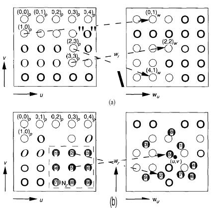
If c is the winning unit, and N,. is the list of unit indices that make up the neighborhood, then the weight-update equations are

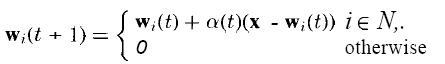
Each weight vector participating in the update process rotates slightly toward the input vector, x. Once training has progressed sufficiently, the weight vector on each unit will converge to a value that is representative of the coordinates of the points near the physical location of the unit.